Chapter 13 Messmer human ESC (Smart-seq2)
13.1 Introduction
This performs an analysis of the human embryonic stem cell (hESC) dataset generated with Smart-seq2 (Messmer et al. 2019), which contains several plates of naive and primed hESCs. The chapter’s code is based on the steps in the paper’s GitHub repository, with some additional steps for cell cycle effect removal contributed by Philippe Boileau.
13.2 Data loading
Converting the batch to a factor, to make life easier later on.
13.3 Quality control
Let’s have a look at the QC statistics.
##              low_lib_size            low_n_features high_subsets_Mito_percent
##                       107                        99                        22
## high_altexps_ERCC_percent                   discard
## 117 156gridExtra::grid.arrange(
plotColData(original, x="experiment batch", y="sum",
colour_by=I(filtered$discard), other_field="phenotype") +
facet_wrap(~phenotype) + scale_y_log10(),
plotColData(original, x="experiment batch", y="detected",
colour_by=I(filtered$discard), other_field="phenotype") +
facet_wrap(~phenotype) + scale_y_log10(),
plotColData(original, x="experiment batch", y="subsets_Mito_percent",
colour_by=I(filtered$discard), other_field="phenotype") +
facet_wrap(~phenotype),
plotColData(original, x="experiment batch", y="altexps_ERCC_percent",
colour_by=I(filtered$discard), other_field="phenotype") +
facet_wrap(~phenotype),
ncol=1
)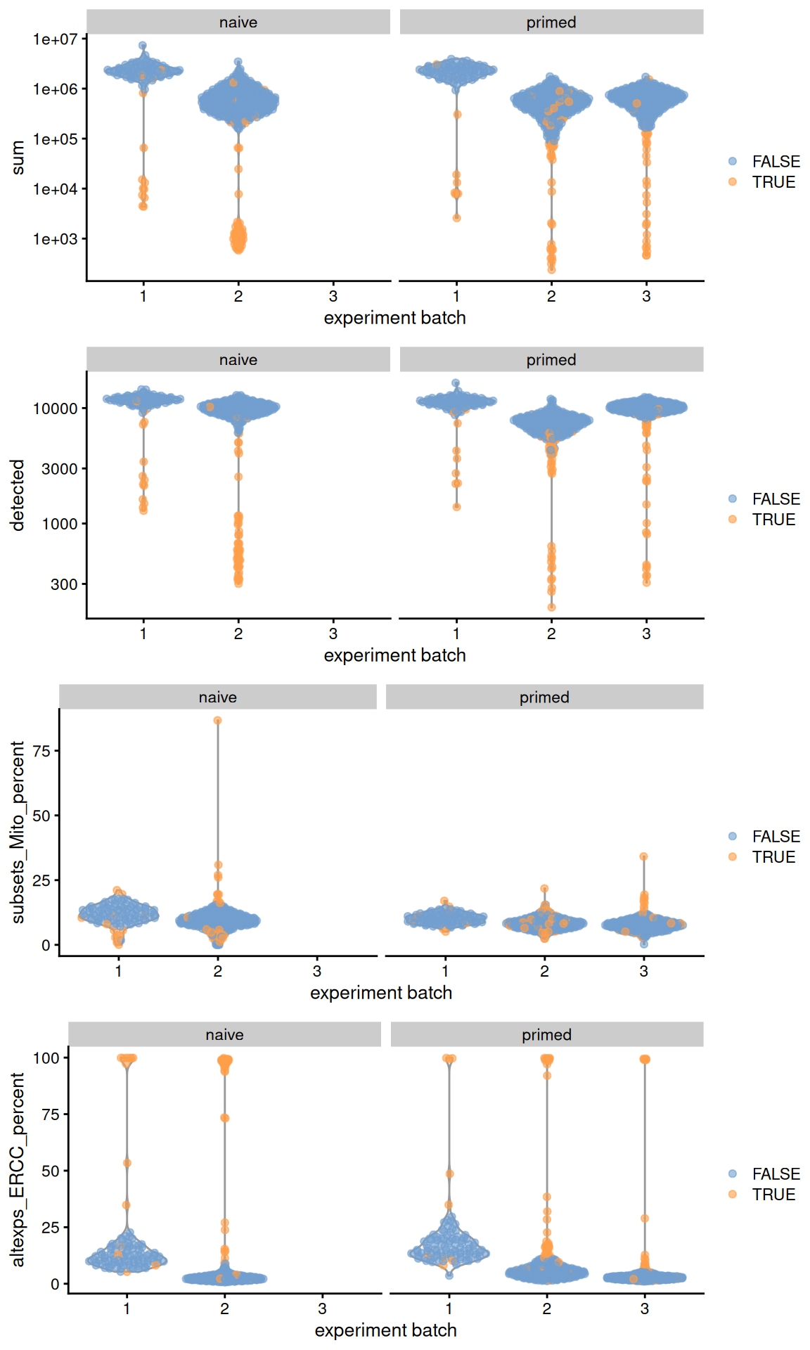
Figure 13.1: Distribution of QC metrics across batches (x-axis) and phenotypes (facets) for cells in the Messmer hESC dataset. Each point is a cell and is colored by whether it was discarded.
13.4 Normalization
library(scran)

set.seed(10000)
clusters <- quickCluster(sce.mess)
sce.mess <- computeSumFactors(sce.mess, cluster=clusters)
sce.mess <- logNormCounts(sce.mess)par(mfrow=c(1,2))
plot(sce.mess$sum, sizeFactors(sce.mess), log = "xy", pch=16,
xlab = "Library size (millions)", ylab = "Size factor",
col = ifelse(sce.mess$phenotype == "naive", "black", "grey"))
spike.sf <- librarySizeFactors(altExp(sce.mess, "ERCC"))
plot(sizeFactors(sce.mess), spike.sf, log = "xy", pch=16,
ylab = "Spike-in size factor", xlab = "Deconvolution size factor",
col = ifelse(sce.mess$phenotype == "naive", "black", "grey"))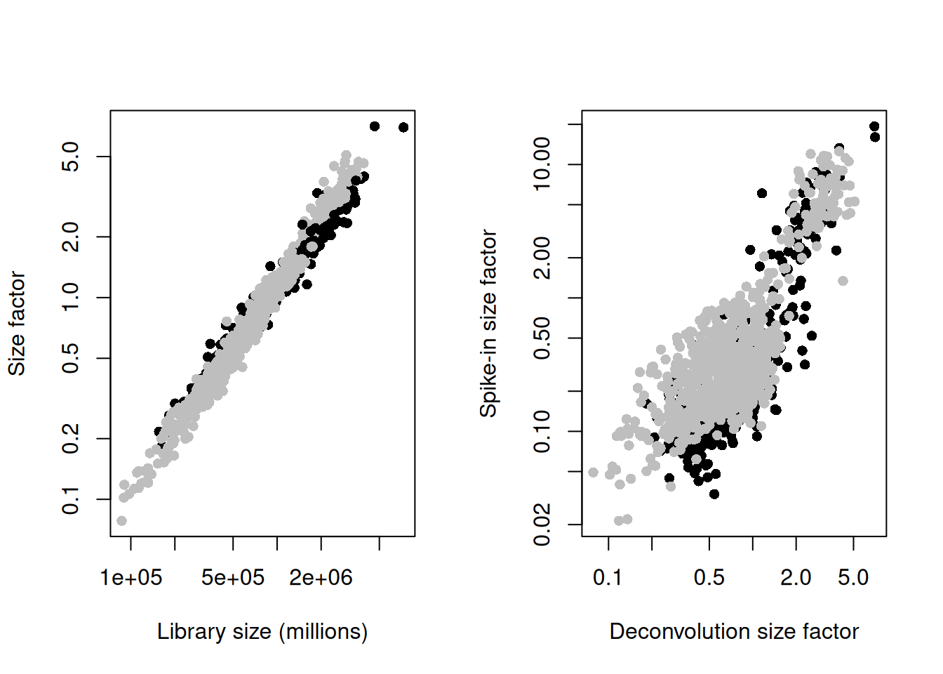
Figure 13.2: Deconvolution size factors plotted against the library size (left) and spike-in size factors plotted against the deconvolution size factors (right). Each point is a cell and is colored by its phenotype.
13.5 Cell cycle phase assignment
Here, we use multiple cores to speed up the processing.
set.seed(10001)
hs_pairs <- readRDS(system.file("exdata", "human_cycle_markers.rds", package="scran"))
assigned <- cyclone(sce.mess, pairs=hs_pairs,
    gene.names=rownames(sce.mess),
    BPPARAM=BiocParallel::MulticoreParam(10))
sce.mess$phase <- assigned$phases##
## G1 G2M S
## 460 406 322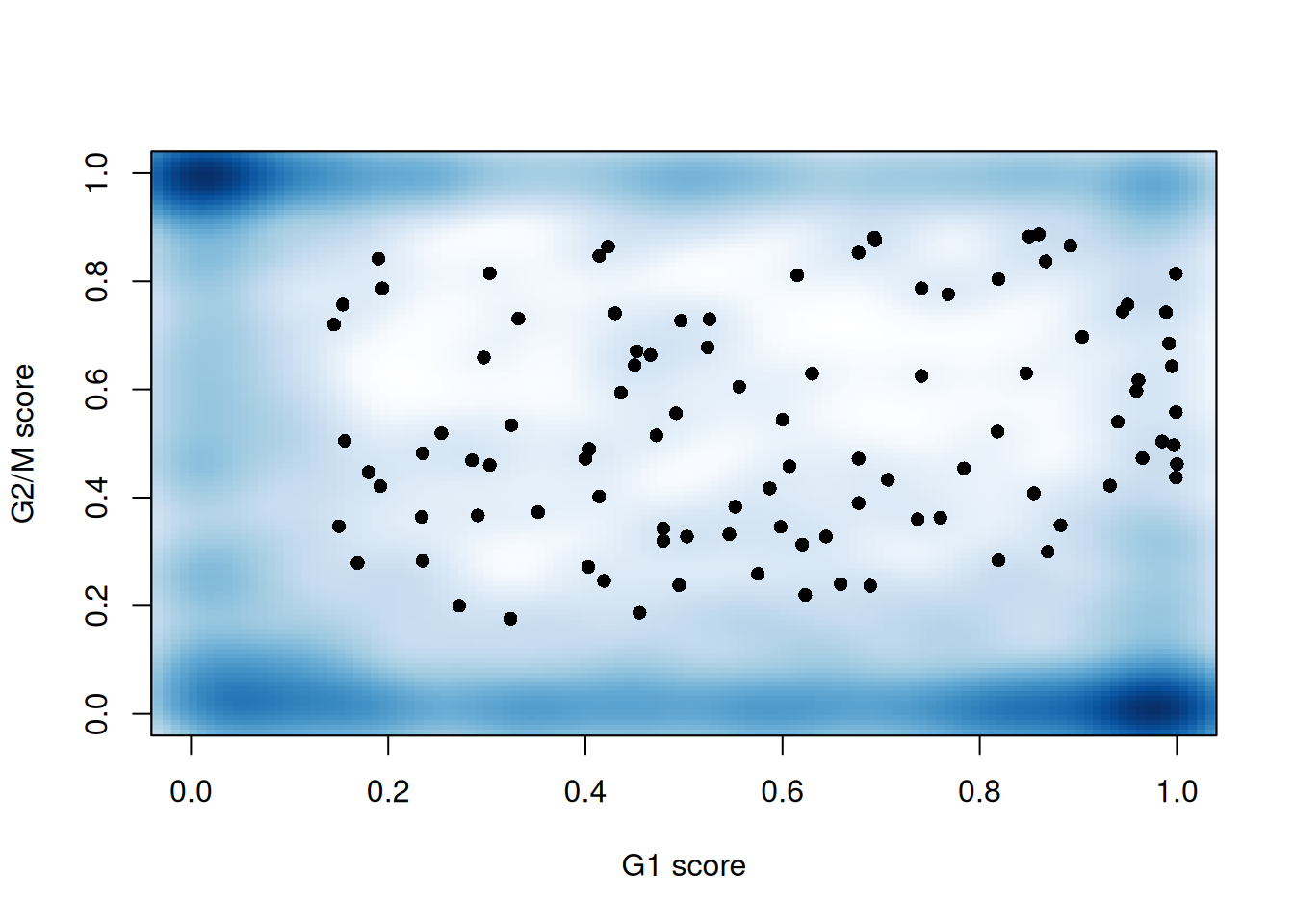
Figure 13.3: G1 cyclone() phase scores against the G2/M phase scores for each cell in the Messmer hESC dataset.
13.6 Feature selection
dec <- modelGeneVarWithSpikes(sce.mess, "ERCC", block = sce.mess$`experiment batch`)
top.hvgs <- getTopHVGs(dec, prop = 0.1)par(mfrow=c(1,3))
for (i in seq_along(dec$per.block)) {
current <- dec$per.block[[i]]
plot(current$mean, current$total, xlab="Mean log-expression",
ylab="Variance", pch=16, cex=0.5, main=paste("Batch", i))
fit <- metadata(current)
points(fit$mean, fit$var, col="red", pch=16)
curve(fit$trend(x), col='dodgerblue', add=TRUE, lwd=2)
}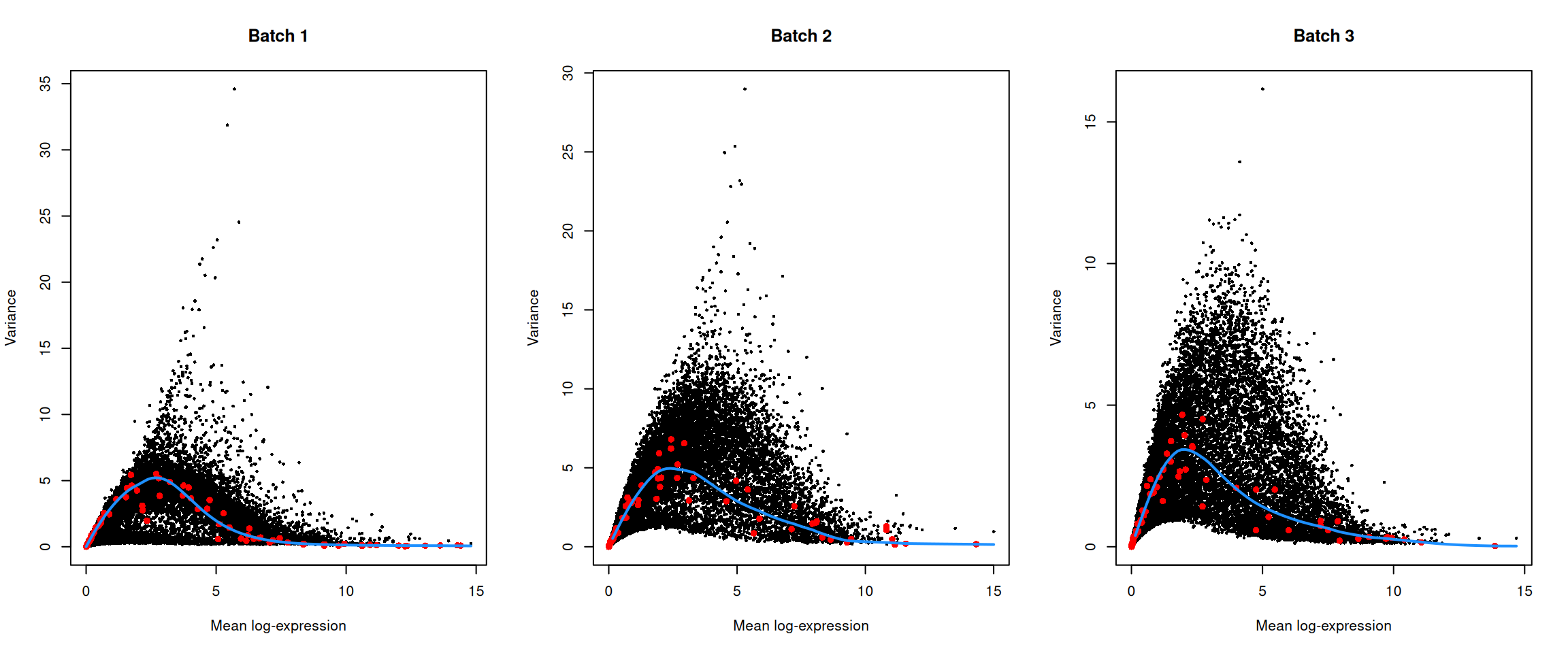
Figure 13.4: Per-gene variance of the log-normalized expression values in the Messmer hESC dataset, plotted against the mean for each batch. Each point represents a gene with spike-ins shown in red and the fitted trend shown in blue.
13.7 Batch correction
We eliminate the obvious batch effect between batches with linear regression, which is possible due to the replicated nature of the experimental design.
We set keep=1:2 to retain the effect of the first two coefficients in design corresponding to our phenotype of interest.
13.8 Dimensionality Reduction
We could have set d= and subset.row= in correctExperiments() to automatically perform a PCA on the the residual matrix with the subset of HVGs,
but we’ll just explicitly call runPCA() here to keep things simple.
set.seed(1101001)
sce.mess <- runPCA(sce.mess, subset_row = top.hvgs, exprs_values = "corrected")
sce.mess <- runTSNE(sce.mess, dimred = "PCA", perplexity = 40)
From a naive PCA, the cell cycle appears to be a major source of biological variation within each phenotype.
gridExtra::grid.arrange(
    plotTSNE(sce.mess, colour_by = "phenotype") + ggtitle("By phenotype"),
    plotTSNE(sce.mess, colour_by = "experiment batch") + ggtitle("By batch "),
    plotTSNE(sce.mess, colour_by = "CDK1", swap_rownames="SYMBOL") + ggtitle("By CDK1"),
    plotTSNE(sce.mess, colour_by = "phase") + ggtitle("By phase"),
    ncol = 2
)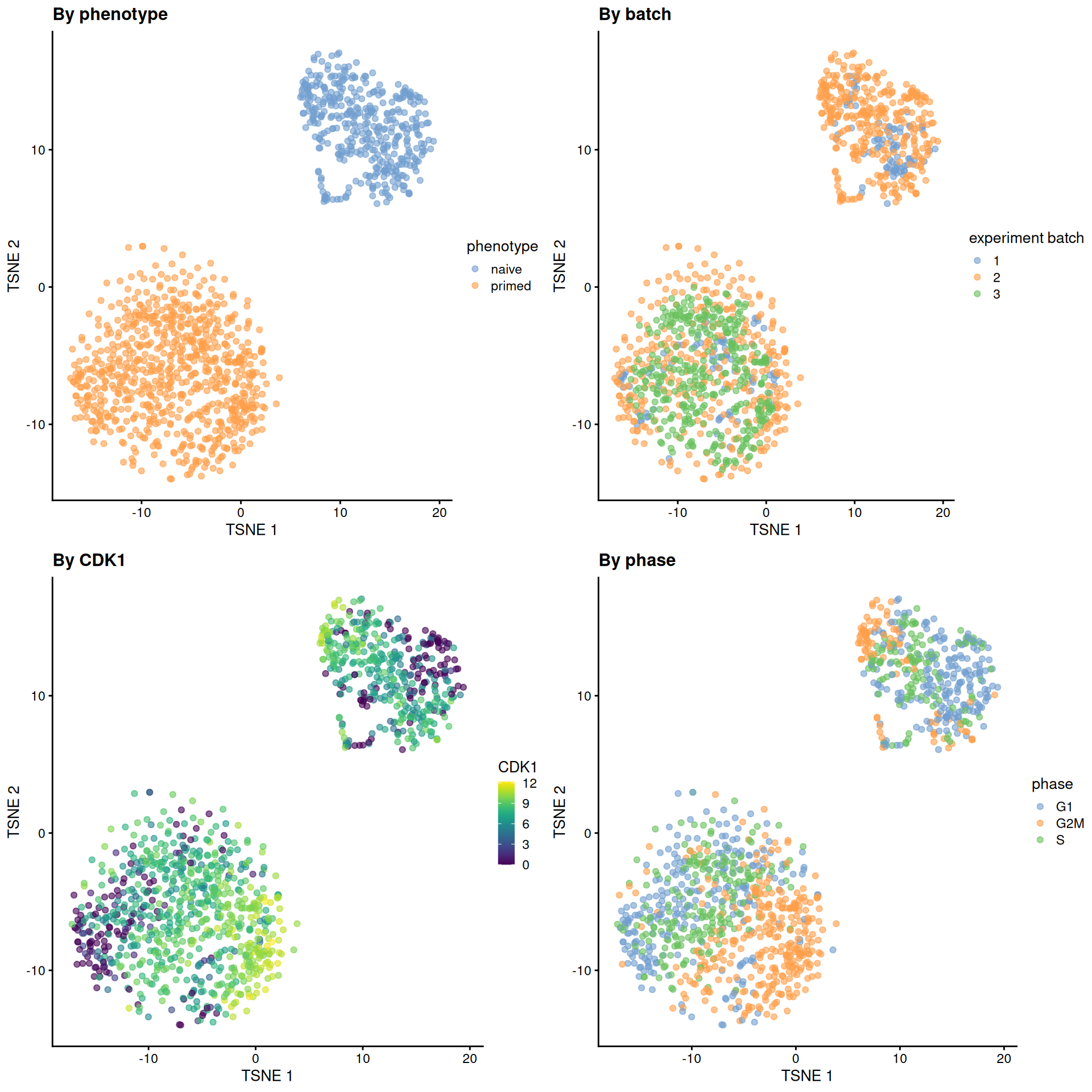
Figure 13.5: Obligatory \(t\)-SNE plots of the Messmer hESC dataset, where each point is a cell and is colored by various attributes.
We perform contrastive PCA (cPCA) and sparse cPCA (scPCA) on the corrected log-expression data to obtain the same number of PCs. Given that the naive hESCs are actually reprogrammed primed hESCs, we will use the single batch of primed-only hESCs as the “background” dataset to remove the cell cycle effect.
library(scPCA)
is.bg <- sce.mess$`experiment batch`=="3"
target <- sce.mess[,!is.bg]
background <- sce.mess[,is.bg]

mat.target <- t(assay(target, "corrected")[top.hvgs,])
mat.background <- t(assay(background, "corrected")[top.hvgs,])

set.seed(1010101001)
con_out <- scPCA(
    target = mat.target,
    background = mat.background,
    penalties = 0, # no penalties = non-sparse cPCA.
    n_eigen = 50,
    contrasts = 100
)
reducedDim(target, "cPCA") <- con_out$xset.seed(101010101)
sparse_con_out <- scPCA(
target = mat.target,
background = mat.background,
penalties = 1e-4,
n_eigen = 50,
contrasts = 100,
alg = "rand_var_proj" # for speed.
)
reducedDim(target, "scPCA") <- sparse_con_out$xWe see greater intermingling between phases within both the naive and primed cells after cPCA and scPCA.
set.seed(1101001)
target <- runTSNE(target, dimred = "cPCA", perplexity = 40, name="cPCA+TSNE")
target <- runTSNE(target, dimred = "scPCA", perplexity = 40, name="scPCA+TSNE")gridExtra::grid.arrange(
plotReducedDim(target, "cPCA+TSNE", colour_by = "phase") + ggtitle("After cPCA"),
plotReducedDim(target, "scPCA+TSNE", colour_by = "phase") + ggtitle("After scPCA"),
ncol=2
)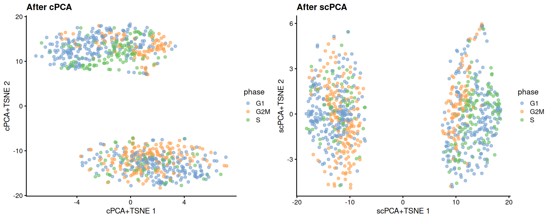
Figure 13.6: More \(t\)-SNE plots of the Messmer hESC dataset after cPCA and scPCA, where each point is a cell and is colored by its assigned cell cycle phase.
We can quantify the change in the separation between phases within each phenotype using the silhouette coefficient.
library(bluster)
naive <- target[,target$phenotype=="naive"]
primed <- target[,target$phenotype=="primed"]

N <- approxSilhouette(reducedDim(naive, "PCA"), naive$phase)
P <- approxSilhouette(reducedDim(primed, "PCA"), primed$phase)
c(naive=mean(N$width), primed=mean(P$width))
## naive primed
## 0.02032 0.03025cN <- approxSilhouette(reducedDim(naive, "cPCA"), naive$phase)
cP <- approxSilhouette(reducedDim(primed, "cPCA"), primed$phase)
c(naive=mean(cN$width), primed=mean(cP$width))## naive primed
## 0.007696 0.011941scN <- approxSilhouette(reducedDim(naive, "scPCA"), naive$phase)
scP <- approxSilhouette(reducedDim(primed, "scPCA"), primed$phase)
c(naive=mean(scN$width), primed=mean(scP$width))## naive primed
## 0.006614 0.014601Session Info
R version 4.6.0 RC (2026-04-17 r89917)
Platform: x86_64-pc-linux-gnu
Running under: Ubuntu 24.04.4 LTS

Matrix products: default
BLAS:   /home/biocbuild/bbs-3.24-bioc/R/lib/libRblas.so
LAPACK: /usr/lib/x86_64-linux-gnu/lapack/liblapack.so.3.12.0  LAPACK version 3.12.0

locale:
 [1] LC_CTYPE=en_US.UTF-8       LC_NUMERIC=C
 [3] LC_TIME=en_GB              LC_COLLATE=C
 [5] LC_MONETARY=en_US.UTF-8    LC_MESSAGES=en_US.UTF-8
 [7] LC_PAPER=en_US.UTF-8       LC_NAME=C
 [9] LC_ADDRESS=C               LC_TELEPHONE=C
[11] LC_MEASUREMENT=en_US.UTF-8 LC_IDENTIFICATION=C

time zone: America/New_York
tzcode source: system (glibc)

attached base packages:
[1] stats4    stats     graphics  grDevices utils     datasets  methods
[8] base

other attached packages:
 [1] bluster_1.23.0              scPCA_1.27.0
 [3] batchelor_1.29.0            scran_1.41.0
 [5] scater_1.41.1               ggplot2_4.0.3
 [7] scuttle_1.23.0              AnnotationHub_4.3.0
 [9] BiocFileCache_3.3.0         dbplyr_2.5.2
[11] ensembldb_2.37.0            AnnotationFilter_1.37.0
[13] GenomicFeatures_1.65.0      AnnotationDbi_1.75.0
[15] scRNAseq_2.27.0             SingleCellExperiment_1.35.0
[17] SummarizedExperiment_1.43.0 Biobase_2.73.1
[19] GenomicRanges_1.65.0        Seqinfo_1.3.0
[21] IRanges_2.47.0              S4Vectors_0.51.1
[23] BiocGenerics_0.59.0         generics_0.1.4
[25] MatrixGenerics_1.25.0       matrixStats_1.5.0
[27] BiocStyle_2.41.0            rebook_1.23.0

loaded via a namespace (and not attached):
  [1] BiocIO_1.23.3             bitops_1.0-9
  [3] filelock_1.0.3            tibble_3.3.1
  [5] CodeDepends_0.6.7         graph_1.91.0
  [7] XML_3.99-0.23             lifecycle_1.0.5
  [9] httr2_1.2.2               Rdpack_2.6.6
 [11] edgeR_4.11.0              globals_0.19.1
 [13] lattice_0.22-9            alabaster.base_1.13.0
 [15] magrittr_2.0.5            limma_3.69.0
 [17] sass_0.4.10               rmarkdown_2.31
 [19] jquerylib_0.1.4           yaml_2.3.12
 [21] metapod_1.21.0            otel_0.2.0
 [23] cowplot_1.2.0             DBI_1.3.0
 [25] RColorBrewer_1.1-3        ResidualMatrix_1.23.0
 [27] abind_1.4-8               Rtsne_0.17
 [29] purrr_1.2.2               RCurl_1.98-1.18
 [31] rappdirs_0.3.4            ggrepel_0.9.8
 [33] irlba_2.3.7               listenv_0.10.1
 [35] alabaster.sce_1.13.0      RSpectra_0.16-2
 [37] parallelly_1.47.0         dqrng_0.4.1
 [39] DelayedMatrixStats_1.35.0 codetools_0.2-20
 [41] DelayedArray_0.39.1       tidyselect_1.2.1
 [43] UCSC.utils_1.9.0          farver_2.1.2
 [45] ScaledMatrix_1.21.0       viridis_0.6.5
 [47] GenomicAlignments_1.49.0  jsonlite_2.0.0
 [49] BiocNeighbors_2.7.0       tools_4.6.0
 [51] Rcpp_1.1.1-1.1            glue_1.8.1
 [53] gridExtra_2.3             SparseArray_1.13.2
 [55] BiocBaseUtils_1.15.0      xfun_0.57
 [57] GenomeInfoDb_1.49.0       dplyr_1.2.1
 [59] HDF5Array_1.41.0          gypsum_1.9.0
 [61] withr_3.0.2               BiocManager_1.30.27
 [63] fastmap_1.2.0             sparsepca_0.1.2
 [65] rhdf5filters_1.25.0       digest_0.6.39
 [67] rsvd_1.0.5                R6_2.6.1
 [69] dichromat_2.0-0.1         RSQLite_2.4.6
 [71] cigarillo_1.3.0           h5mread_1.5.0
 [73] data.table_1.18.2.1       rtracklayer_1.73.0
 [75] httr_1.4.8                S4Arrays_1.13.0
 [77] pkgconfig_2.0.3           gtable_0.3.6
 [79] blob_1.3.0                S7_0.2.2
 [81] XVector_0.53.0            htmltools_0.5.9
 [83] bookdown_0.46             ProtGenerics_1.45.0
 [85] scales_1.4.0              alabaster.matrix_1.13.0
 [87] png_0.1-9                 knitr_1.51
 [89] rjson_0.2.23              curl_7.1.0
 [91] cachem_1.1.0              rhdf5_2.57.0
 [93] stringr_1.6.0             BiocVersion_3.24.0
 [95] KernSmooth_2.23-26        parallel_4.6.0
 [97] vipor_0.4.7               restfulr_0.0.16
 [99] pillar_1.11.1             grid_4.6.0
[101] alabaster.schemas_1.13.0  vctrs_0.7.3
[103] origami_1.0.7             BiocSingular_1.29.0
[105] beachmat_2.29.0           cluster_2.1.8.2
[107] beeswarm_0.4.0            evaluate_1.0.5
[109] cli_3.6.6                 locfit_1.5-9.12
[111] compiler_4.6.0            Rsamtools_2.29.0
[113] rlang_1.2.0               crayon_1.5.3
[115] future.apply_1.20.2       labeling_0.4.3
[117] ggbeeswarm_0.7.3          stringi_1.8.7
[119] alabaster.se_1.13.0       viridisLite_0.4.3
[121] BiocParallel_1.47.0       assertthat_0.2.1
[123] Biostrings_2.81.1         coop_0.6-3
[125] lazyeval_0.2.3            Matrix_1.7-5
[127] dir.expiry_1.21.0         ExperimentHub_3.3.0
[129] future_1.70.0             sparseMatrixStats_1.25.0
[131] bit64_4.8.0               Rhdf5lib_2.1.0
[133] KEGGREST_1.53.0           statmod_1.5.1
[135] alabaster.ranges_1.13.0   kernlab_0.9-33
[137] rbibutils_2.4.1           igraph_2.3.1
[139] memoise_2.0.1             bslib_0.10.0
[141] bit_4.6.0
References
Messmer, T., F. von Meyenn, A. Savino, F. Santos, H. Mohammed, A. T. L. Lun, J. C. Marioni, and W. Reik. 2019. “Transcriptional heterogeneity in naive and primed human pluripotent stem cells at single-cell resolution.” Cell Rep 26 (4): 815–24.