Chapter 3 Unfiltered human PBMCs (10X Genomics)
3.1 Introduction
Here, we describe a brief analysis of the peripheral blood mononuclear cell (PBMC) dataset from 10X Genomics (Zheng et al. 2017). The data are publicly available from the 10X Genomics website, from which we download the raw gene/barcode count matrices, i.e., before cell calling from the CellRanger pipeline.
3.2 Data loading
3.3 Quality control
We perform cell detection using the emptyDrops() algorithm, as discussed in Advanced Section 7.2.
set.seed(100)
e.out <- emptyDrops(counts(sce.pbmc))
sce.pbmc <- sce.pbmc[,which(e.out$FDR <= 0.001)]We use a relaxed QC strategy and only remove cells with large mitochondrial proportions, using it as a proxy for cell damage. This reduces the risk of removing cell types with low RNA content, especially in a heterogeneous PBMC population with many different cell types.
stats <- perCellQCMetrics(sce.pbmc, subsets=list(Mito=which(location=="MT")))
high.mito <- isOutlier(stats$subsets_Mito_percent, type="higher")
sce.pbmc <- sce.pbmc[,!high.mito]## Mode FALSE TRUE
## logical 3985 315colData(unfiltered) <- cbind(colData(unfiltered), stats)
unfiltered$discard <- high.mito
gridExtra::grid.arrange(
plotColData(unfiltered, y="sum", colour_by="discard") +
scale_y_log10() + ggtitle("Total count"),
plotColData(unfiltered, y="detected", colour_by="discard") +
scale_y_log10() + ggtitle("Detected features"),
plotColData(unfiltered, y="subsets_Mito_percent",
colour_by="discard") + ggtitle("Mito percent"),
ncol=2
)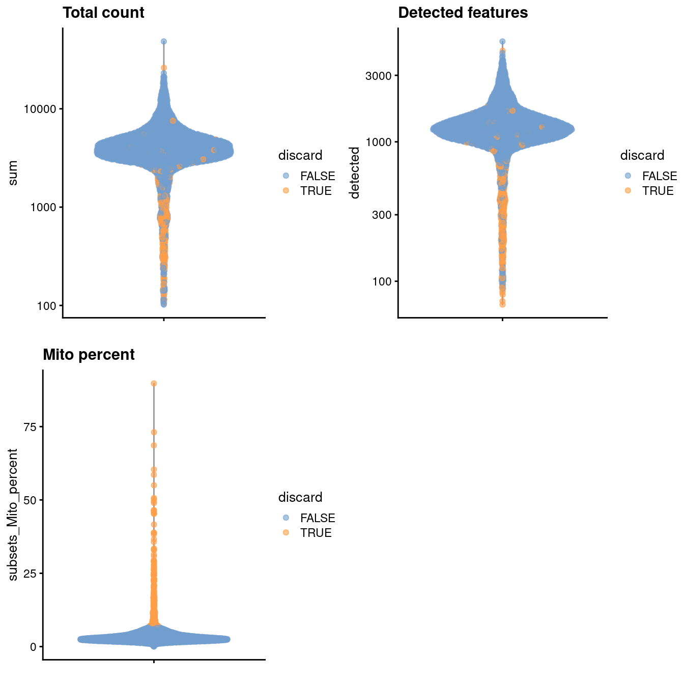
Figure 3.1: Distribution of various QC metrics in the PBMC dataset after cell calling. Each point is a cell and is colored according to whether it was discarded by the mitochondrial filter.
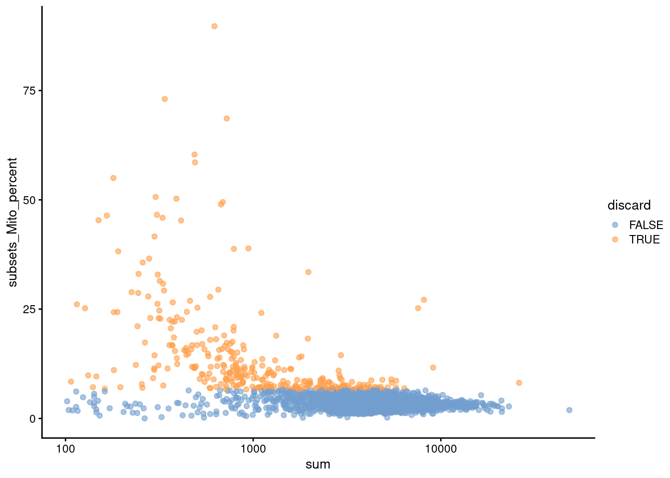
Figure 3.2: Proportion of mitochondrial reads in each cell of the PBMC dataset compared to its total count.
3.4 Normalization
library(scran)
set.seed(1000)
clusters <- quickCluster(sce.pbmc)
sce.pbmc <- computeSumFactors(sce.pbmc, cluster=clusters)
sce.pbmc <- logNormCounts(sce.pbmc)## Min. 1st Qu. Median Mean 3rd Qu. Max.
## 0.007 0.712 0.875 1.000 1.099 12.254plot(librarySizeFactors(sce.pbmc), sizeFactors(sce.pbmc), pch=16,
xlab="Library size factors", ylab="Deconvolution factors", log="xy")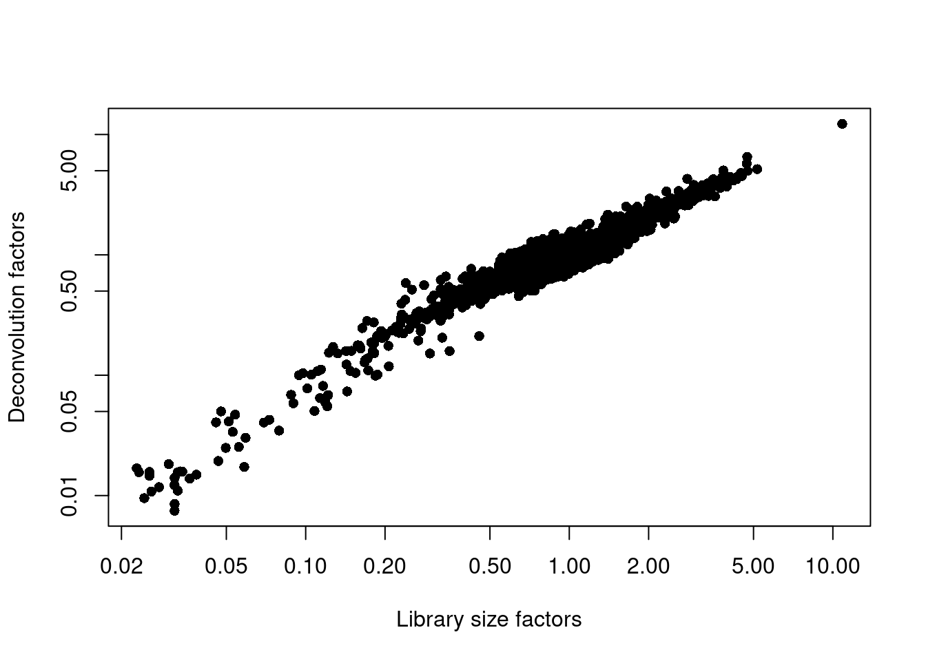
Figure 3.3: Relationship between the library size factors and the deconvolution size factors in the PBMC dataset.
3.5 Variance modelling
set.seed(1001)
dec.pbmc <- modelGeneVarByPoisson(sce.pbmc)
top.pbmc <- getTopHVGs(dec.pbmc, prop=0.1)plot(dec.pbmc$mean, dec.pbmc$total, pch=16, cex=0.5,
xlab="Mean of log-expression", ylab="Variance of log-expression")
curfit <- metadata(dec.pbmc)
curve(curfit$trend(x), col='dodgerblue', add=TRUE, lwd=2)
Figure 3.4: Per-gene variance as a function of the mean for the log-expression values in the PBMC dataset. Each point represents a gene (black) with the mean-variance trend (blue) fitted to simulated Poisson counts.
3.6 Dimensionality reduction
set.seed(10000)
sce.pbmc <- denoisePCA(sce.pbmc, subset.row=top.pbmc, technical=dec.pbmc)

set.seed(100000)
sce.pbmc <- runTSNE(sce.pbmc, dimred="PCA")

set.seed(1000000)
sce.pbmc <- runUMAP(sce.pbmc, dimred="PCA")
We verify that a reasonable number of PCs is retained.
## [1] 93.7 Clustering
g <- buildSNNGraph(sce.pbmc, k=10, use.dimred = 'PCA')
clust <- igraph::cluster_walktrap(g)$membership
colLabels(sce.pbmc) <- factor(clust)##
## 1 2 3 4 5 6 7 8 9 10 11 12 13 14 15 16
## 205 508 541 56 374 125 46 432 302 867 47 155 166 61 84 16
Figure 3.5: Obligatory \(t\)-SNE plot of the PBMC dataset, where each point represents a cell and is colored according to the assigned cluster.
3.8 Interpretation
We examine the markers for cluster 8 in more detail. High expression of CD14, CD68 and MNDA combined with low expression of CD16 suggests that this cluster contains monocytes, compared to macrophages in cluster 15 (Figure 3.6).
##                  p.value        FDR summary.logFC
## CSTA          7.171e-222 2.016e-217        2.4179
## MNDA          1.197e-221 2.016e-217        2.6615
## FCN1          2.376e-213 2.669e-209        2.6381
## S100A12       4.393e-212 3.701e-208        3.0809
## VCAN          1.711e-199 1.153e-195        2.2604
## TYMP          1.174e-154 6.590e-151        2.0238
## AIF1          3.674e-149 1.768e-145        2.4604
## LGALS2        4.005e-137 1.687e-133        1.8928
## MS4A6A        5.640e-134 2.111e-130        1.5457
## FGL2          2.045e-124 6.889e-121        1.3859
## RP11-1143G9.4 6.892e-122 2.111e-118        2.8042
## AP1S2         1.786e-112 5.015e-109        1.7704
## CD14          1.195e-110 3.098e-107        1.4260
## CFD           6.870e-109 1.654e-105        1.3560
## GPX1          9.049e-107 2.033e-103        2.4014
## TNFSF13B       3.920e-95  8.256e-92        1.1151
## KLF4           3.310e-94  6.560e-91        1.2049
## GRN            4.801e-91  8.987e-88        1.3815
## NAMPT          2.490e-90  4.415e-87        1.1439
## CLEC7A         7.736e-88  1.303e-84        1.0616
## S100A8         3.125e-84  5.014e-81        4.8052
## SERPINA1       1.580e-82  2.420e-79        1.3843
## CD36           8.018e-79  1.175e-75        1.0538
## MPEG1          8.482e-79  1.191e-75        0.9778
## CD68           5.119e-78  6.899e-75        0.9481
## CYBB           1.201e-77  1.556e-74        1.0300
## S100A11        1.175e-72  1.466e-69        1.8962
## RBP7           2.467e-71  2.969e-68        0.9666
## BLVRB          3.763e-71  4.372e-68        0.9701
## CD302 9.859e-71 1.107e-67 0.8792plotExpression(sce.pbmc, features=c("CD14", "CD68",
"MNDA", "FCGR3A"), x="label", colour_by="label")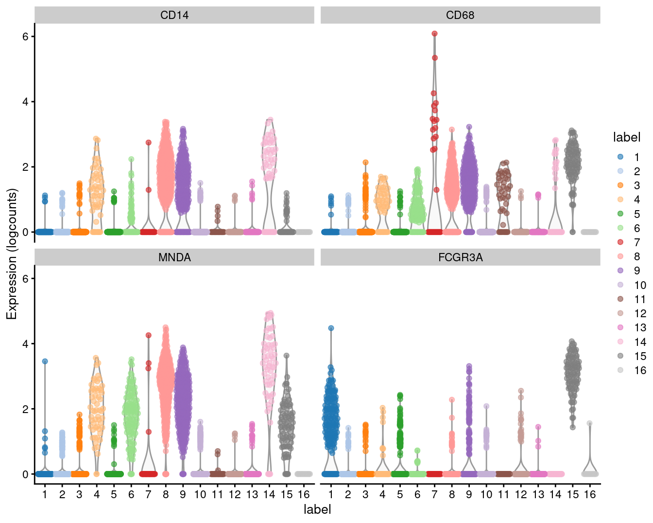
Figure 3.6: Distribution of expression values for monocyte and macrophage markers across clusters in the PBMC dataset.
Session Info
R version 4.1.1 (2021-08-10)
Platform: x86_64-pc-linux-gnu (64-bit)
Running under: Ubuntu 20.04.3 LTS

Matrix products: default
BLAS:   /home/biocbuild/bbs-3.14-bioc/R/lib/libRblas.so
LAPACK: /home/biocbuild/bbs-3.14-bioc/R/lib/libRlapack.so

locale:
 [1] LC_CTYPE=en_US.UTF-8       LC_NUMERIC=C
 [3] LC_TIME=en_GB              LC_COLLATE=C
 [5] LC_MONETARY=en_US.UTF-8    LC_MESSAGES=en_US.UTF-8
 [7] LC_PAPER=en_US.UTF-8       LC_NAME=C
 [9] LC_ADDRESS=C               LC_TELEPHONE=C
[11] LC_MEASUREMENT=en_US.UTF-8 LC_IDENTIFICATION=C

attached base packages:
[1] stats4    stats     graphics  grDevices utils     datasets  methods
[8] base

other attached packages:
 [1] scran_1.22.0                EnsDb.Hsapiens.v86_2.99.0
 [3] ensembldb_2.18.0            AnnotationFilter_1.18.0
 [5] GenomicFeatures_1.46.0      AnnotationDbi_1.56.0
 [7] scater_1.22.0               ggplot2_3.3.5
 [9] scuttle_1.4.0               DropletUtils_1.14.0
[11] SingleCellExperiment_1.16.0 SummarizedExperiment_1.24.0
[13] Biobase_2.54.0              GenomicRanges_1.46.0
[15] GenomeInfoDb_1.30.0         IRanges_2.28.0
[17] S4Vectors_0.32.0            BiocGenerics_0.40.0
[19] MatrixGenerics_1.6.0        matrixStats_0.61.0
[21] DropletTestFiles_1.3.0      BiocStyle_2.22.0
[23] rebook_1.4.0

loaded via a namespace (and not attached):
  [1] AnnotationHub_3.2.0           BiocFileCache_2.2.0
  [3] igraph_1.2.7                  lazyeval_0.2.2
  [5] BiocParallel_1.28.0           digest_0.6.28
  [7] htmltools_0.5.2               viridis_0.6.2
  [9] fansi_0.5.0                   magrittr_2.0.1
 [11] memoise_2.0.0                 ScaledMatrix_1.2.0
 [13] cluster_2.1.2                 limma_3.50.0
 [15] Biostrings_2.62.0             R.utils_2.11.0
 [17] prettyunits_1.1.1             colorspace_2.0-2
 [19] blob_1.2.2                    rappdirs_0.3.3
 [21] ggrepel_0.9.1                 xfun_0.27
 [23] dplyr_1.0.7                   crayon_1.4.1
 [25] RCurl_1.98-1.5                jsonlite_1.7.2
 [27] graph_1.72.0                  glue_1.4.2
 [29] gtable_0.3.0                  zlibbioc_1.40.0
 [31] XVector_0.34.0                DelayedArray_0.20.0
 [33] BiocSingular_1.10.0           Rhdf5lib_1.16.0
 [35] HDF5Array_1.22.0              scales_1.1.1
 [37] DBI_1.1.1                     edgeR_3.36.0
 [39] Rcpp_1.0.7                    viridisLite_0.4.0
 [41] xtable_1.8-4                  progress_1.2.2
 [43] dqrng_0.3.0                   bit_4.0.4
 [45] rsvd_1.0.5                    metapod_1.2.0
 [47] httr_1.4.2                    FNN_1.1.3
 [49] dir.expiry_1.2.0              ellipsis_0.3.2
 [51] farver_2.1.0                  pkgconfig_2.0.3
 [53] XML_3.99-0.8                  R.methodsS3_1.8.1
 [55] uwot_0.1.10                   CodeDepends_0.6.5
 [57] sass_0.4.0                    dbplyr_2.1.1
 [59] locfit_1.5-9.4                utf8_1.2.2
 [61] labeling_0.4.2                tidyselect_1.1.1
 [63] rlang_0.4.12                  later_1.3.0
 [65] munsell_0.5.0                 BiocVersion_3.14.0
 [67] tools_4.1.1                   cachem_1.0.6
 [69] generics_0.1.1                RSQLite_2.2.8
 [71] ExperimentHub_2.2.0           evaluate_0.14
 [73] stringr_1.4.0                 fastmap_1.1.0
 [75] yaml_2.2.1                    knitr_1.36
 [77] bit64_4.0.5                   purrr_0.3.4
 [79] KEGGREST_1.34.0               sparseMatrixStats_1.6.0
 [81] mime_0.12                     R.oo_1.24.0
 [83] xml2_1.3.2                    biomaRt_2.50.0
 [85] compiler_4.1.1                beeswarm_0.4.0
 [87] filelock_1.0.2                curl_4.3.2
 [89] png_0.1-7                     interactiveDisplayBase_1.32.0
 [91] statmod_1.4.36                tibble_3.1.5
 [93] bslib_0.3.1                   stringi_1.7.5
 [95] highr_0.9                     RSpectra_0.16-0
 [97] bluster_1.4.0                 lattice_0.20-45
 [99] ProtGenerics_1.26.0           Matrix_1.3-4
[101] vctrs_0.3.8                   pillar_1.6.4
[103] lifecycle_1.0.1               rhdf5filters_1.6.0
[105] BiocManager_1.30.16           jquerylib_0.1.4
[107] BiocNeighbors_1.12.0          cowplot_1.1.1
[109] bitops_1.0-7                  irlba_2.3.3
[111] rtracklayer_1.54.0            httpuv_1.6.3
[113] R6_2.5.1                      BiocIO_1.4.0
[115] bookdown_0.24                 promises_1.2.0.1
[117] gridExtra_2.3                 vipor_0.4.5
[119] codetools_0.2-18              assertthat_0.2.1
[121] rhdf5_2.38.0                  rjson_0.2.20
[123] withr_2.4.2                   GenomicAlignments_1.30.0
[125] Rsamtools_2.10.0              GenomeInfoDbData_1.2.7
[127] parallel_4.1.1                hms_1.1.1
[129] grid_4.1.1                    beachmat_2.10.0
[131] rmarkdown_2.11                DelayedMatrixStats_1.16.0
[133] Rtsne_0.15                    shiny_1.7.1
[135] ggbeeswarm_0.6.0              restfulr_0.0.13
References
Zheng, G. X., J. M. Terry, P. Belgrader, P. Ryvkin, Z. W. Bent, R. Wilson, S. B. Ziraldo, et al. 2017. “Massively parallel digital transcriptional profiling of single cells.” Nat Commun 8 (January): 14049.