---
title: 'Low-dimensional embeddings 1'
author: "Levi Waldron"
output: slidy_presentation
---

```{r setup, include=FALSE}
knitr::opts_chunk$set(eval = TRUE, cache=FALSE)
```

## Outline

Based on [Biomedical Data Science](https://genomicsclass.github.io/book/) by Irizarry and Love, chapter 8.

-   Distances in high dimensions
-   Principal Components Analysis and Singular Value Decomposition
-   Multidimensional Scaling (Principal Coordinates Analysis)
-   GenomicSuperSignatures Bioconductor package

Built slides at https://rpubs.com/lwaldron/916521

## Metrics and distances

A **metric** satisfies the following five properties:

1.  non-negativity $d(a, b) \ge 0$
2.  symmetry $d(a, b) = d(b, a)$
3.  identification mark $d(a, a) = 0$
4.  definiteness $d(a, b) = 0$ if and only if $a=b$
5.  triangle inequality $d(a, b) + d(b, c) \ge d(a, c)$

-   A **similarity function** satisfies 1-2, and **increases** as $a$ and $b$ become more similar
-   A **dissimilarity function** satisfies 1-2, and **decreases** as $a$ and $b$ become more similar

## Euclidian distance (metric)

-   Remember grade school:

```{r, echo=FALSE, fig.height=3.5}
rafalib::mypar()
plot(
    c(0, 1, 1),
    c(0, 0, 1),
    pch = 16,
    cex = 2,
    xaxt = "n",
    yaxt = "n",
    xlab = "",
    ylab = "",
    bty = "n",
    xlim = c(-0.25, 1.25),
    ylim = c(-0.25, 1.25)
)
lines(c(0, 1, 1, 0), c(0, 0, 1, 0))
text(0, .2, expression(paste('(A'[x] * ',A'[y] * ')')), cex = 1.5)
text(1, 1.2, expression(paste('(B'[x] * ',B'[y] * ')')), cex = 1.5)
text(-0.1, 0, "A", cex = 2)
text(1.1, 1, "B", cex = 2)
```

<center>

Euclidean d = $\sqrt{ (A_x-B_x)^2 + (A_y-B_y)^2}$.

</center>

-   **Side note**: also referred to as $L_2$ norm

## Euclidian distance in high dimensions

```{r, echo = FALSE, message=FALSE, warning=FALSE}
if(!require(tissuesGeneExpression)){
  BiocManager::install("genomicsclass/tissuesGeneExpression")
}
if(!require(GSE5859)){
  BiocManager::install("genomicsclass/GSE5859")
}
```

```{r}
## BiocManager::install("genomicsclass/tissuesGeneExpression") #if needed
## BiocManager::install("genomicsclass/GSE5859") #if needed
library(GSE5859)
library(tissuesGeneExpression)
data(tissuesGeneExpression)
dim(e) ##gene expression data
table(tissue) ##tissue[i] corresponds to e[,i]
```

Interested in identifying similar *samples* and similar *genes*

## Notes about Euclidian distance in high dimensions

-   Points are no longer on the Cartesian plane
-   instead they are in higher dimensions. For example:
    -   sample $i$ is defined by a point in 22,215 dimensional space: $(Y_{1,i},\dots,Y_{22215,i})^\top$.
    -   feature $g$ is defined by a point in 189 dimensions $(Y_{g,189},\dots,Y_{g,189})^\top$

Euclidean distance as for two dimensions. E.g., the distance between two samples $i$ and $j$ is:

$$ \mbox{dist}(i,j) = \sqrt{ \sum_{g=1}^{22215} (Y_{g,i}-Y_{g,j })^2 } $$

and the distance between two features $h$ and $g$ is:

$$ \mbox{dist}(h,g) = \sqrt{ \sum_{i=1}^{189} (Y_{h,i}-Y_{g,i})^2 } $$

## Euclidian distance in matrix algebra notation

The Euclidian distance between samples $i$ and $j$ can be written as:

$$ \mbox{dist}(i,j) = \sqrt{ (\mathbf{Y}_i - \mathbf{Y}_j)^\top(\mathbf{Y}_i - \mathbf{Y}_j) }$$

with $\mathbf{Y}_i$ and $\mathbf{Y}_j$ columns $i$ and $j$.

```{r}
t(matrix(1:3, ncol = 1))
matrix(1:3, ncol = 1)
t(matrix(1:3, ncol = 1)) %*% matrix(1:3, ncol = 1)
```

## Note about matrix algebra in R

-   R is very efficient at "vectorized" matrix algebra
-   for very large matricies, see the:
    -   [Matrix](https://CRAN.R-project.org/package=Matrix) CRAN package (sparse matrices)
    -   [rhdf5](https://bioconductor.org/packages/rhdf5/) and [DelayedArray](https://bioconductor.org/packages/DelayedArray/) Bioconductor package (on-disk arrays)

## 2-sample example

```{r}
kidney1 <- e[, 1]
kidney2 <- e[, 2]
colon1 <- e[, 87]
sqrt(sum((kidney1 - kidney2) ^ 2))
sqrt(sum((kidney1 - colon1) ^ 2))
```

## 3-sample example using dist()

```{r}
dim(e)
(d <- dist(t(e[, c(1, 2, 87)])))
class(d)
```

## The dist() function

Excerpt from ?dist:

```{r, eval=FALSE}
dist(x,
    method = "euclidean",
    diag = FALSE,
    upper = FALSE,
    p = 2)
```

-   **method:** the distance measure to be used.
    -   This must be one of "euclidean", "maximum", "manhattan", "canberra", "binary" or "minkowski".
-   `dist` class output from `dist()` is used for many clustering algorithms and heatmap functions

*Caution*: `dist(e)` creates a `r nrow(e)` x `r nrow(e)` matrix that will probably crash your R session.

## Note on standardization

-   In practice, features (measures) should usually be "standardized" when calculating distances, for example by converting to z-score:

$$x_{gi} \leftarrow \frac{(x_{gi} - \bar{x}_g)}{s_g}$$

-   This is done because the differences in overall amplitude between features may be technical, *e.g.*:
    -   GC bias, PCR amplification efficiency, ...
-   Euclidian distance and $1-r$ (Pearson cor) are related:
    -   $\frac{d_E(x, y)^2}{2m} = 1 - r_{xy}$
    -   $m$ = \# dimensions

## Dimension reduction and PCA

-   Motivation for dimension reduction

Simulate the heights of twin pairs:

```{r}
set.seed(1)
n <- 100
y <- t(MASS::mvrnorm(n, c(0, 0), matrix(c(1, 0.95, 0.95, 1), 2, 2)))
dim(y)
cor(t(y))
```

## Visualizing twin pairs data

```{r, echo=FALSE}
z1 = (y[1,] + y[2,]) / 2 #the sum
z2 = (y[1,] - y[2,])   #the difference

z = rbind(z1, z2) #matrix now same dimensions as y

thelim <- c(-3, 3)
rafalib::mypar(1, 2)

plot(
    y[1,],
    y[2,],
    xlab = "Twin 1 (standardized height)",
    ylab = "Twin 2 (standardized height)",
    xlim = thelim,
    ylim = thelim,
    main = "Original twin heights"
)
points(y[1, 1:2], y[2, 1:2], col = 2, pch = 16)

plot(
    z[1,],
    z[2,],
    xlim = thelim,
    ylim = thelim,
    xlab = "Average height",
    ylab = "Difference in height",
    main = "Manual PCA-like projection"
)
points(z[1, 1:2] , z[2, 1:2], col = 2, pch = 16)
```

## Not much distance is lost in the second dimension

```{r, echo=FALSE}
rafalib::mypar()
d = dist(t(y))
d3 = dist(z[1, ]) * sqrt(2) ##distance computed using just first dimension mypar(1,1)
plot(as.numeric(d),
     as.numeric(d3),
     xlab = "Pairwise distances in 2 dimensions",
     ylab = "Pairwise distances in 1 dimension")
abline(0, 1, col = "red")
```

-   Not much loss of height differences when just using average heights of twin pairs.
    -   because twin heights are highly correlated

## Singular Value Decomposition (SVD)

SVD generalizes the example rotation we looked at:

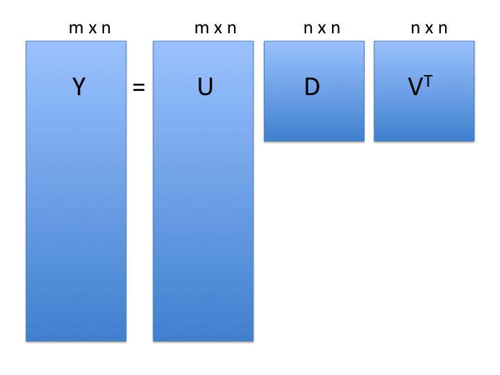
$$\mathbf{Y} = \mathbf{UDV}^\top$$

<center>

<img src="lecture-02-figures/SVD1.png" alt="SVD" align="middle" style="height: 350px;"/>

</center>

-   **note**: the above formulation is for $m$ rows $> n$ columns

-   $\mathbf{Y}$: the $m$ rows x $n$ cols matrix of measurements

-   $\mathbf{U}$: $m \times n$ matrix relating original scores to PCA scores (**loadings**)

-   $\mathbf{D}$: $n \times n$ diagonal matrix (**eigenvalues**)

-   $\mathbf{V}$: $n \times n$ *orthogonal* matrix (**eigenvectors or PCA scores**)

    -   orthogonal = unit length and "perpendicular" in 3-D

## SVD of gene expression dataset

Scaling:

```{r}
e.standardized <- t(scale(t(e), center = TRUE, scale = FALSE))
```

SVD:

```{r}
s <- svd(e.standardized)
names(s)
```

## Components of SVD results

```{r}
dim(s$u)     # loadings
length(s$d)  # eigenvalues
dim(s$v)     # d %*% vT = scores
```

<center>

<img src="lecture-02-figures/SVD1.png" alt="SVD" align="middle" style="height: 200px;"/>

</center>

## PCA is a SVD

-   gene expression dataset

```{r, cache=TRUE}
rafalib::mypar()
p <- prcomp(t(e.standardized))
plot(s$u[, 1] ~ p$rotation[, 1])
```

**Lesson:** u and v can each be multiplied by -1 arbitrarily

## PCA interpretation: loadings

<center>

<img src="lecture-02-figures/SVD1.png" alt="SVD" align="middle" style="height: 225px;"/>

</center>

-   $\mathbf{U}$ (**loadings**): relate the *principal component* axes to the original variables
    -   think of principal component axes as a weighted combination of original axes

## Visualizing PCA loadings

```{r}
plot(p$rotation[, 1],
     xlab = "Index of genes",
     ylab = "Loadings of PC1",
     main = "PC1 loadings of each gene")
abline(h = c(-0.03, 0.03), col = "red")
```

## Genes with high PC1 loadings

```{r, fig.height=3.5}
e.pc1genes <-
    e.standardized[p$rotation[, 1] < -0.03 |
                           p$rotation[, 1] > 0.03,]
dim(e.pc1genes)
```

```{r, echo = FALSE}
pheatmap::pheatmap(
    e.pc1genes,
    scale = "none",
    show_rownames = TRUE,
    show_colnames = FALSE
)
```

## PCA interpretation: eigenvalues

-   $\mathbf{D}$ (**eigenvalues**): standard deviation scaling factor that each decomposed variable is multiplied by.

```{r, fig.height=3, fig.width=5, echo=TRUE, fig.align='center'}
rafalib::mypar()
plot(
    p$sdev ^ 2 / sum(p$sdev ^ 2) * 100,
    xlim = c(0, 150),
    type = "b",
    ylab = "% variance explained",
    main = "Screeplot"
)
```

## PCA interpretation: eigenvalues

Alternatively as cumulative % variance explained (using `cumsum()` function)

```{r, fig.height=4, echo=TRUE, fig.align='center'}
rafalib::mypar()
plot(
    cumsum(p$sdev ^ 2) / sum(p$sdev ^ 2) * 100,
    ylab = "cumulative % variance explained",
    ylim = c(0, 100),
    type = "b",
    main = "Cumulative screeplot"
)
```

## PCA interpretation: scores

<center>

<img src="lecture-02-figures/SVD1.png" alt="SVD" align="middle" style="height: 225px;"/>

</center>

-   $\mathbf{V}$ (**scores**): The "datapoints" in the reduced prinipal component space
-   In some implementations (like `prcomp()`), scores are already scaled by eigenvalues: $\mathbf{D V^T}$

## PCA interpretation: scores

```{r, fig.height=5, echo=FALSE}
rafalib::mypar()
plot(
    p$x[, 1:2],
    xlab = "PC1",
    ylab = "PC2",
    main = "plot of p$x[, 1:2]",
    col = factor(tissue),
    pch = as.integer(factor(tissue))
)
legend(
    "topright",
    legend = levels(factor(tissue)),
    col = 1:length(unique(tissue)),
    pch = 1:length(unique(tissue)),
    bty = 'n'
)
```

## Multi-dimensional Scaling (MDS)

-   also referred to as Principal Coordinates Analysis (PCoA)
-   a reduced SVD, performed on a distance matrix
-   identify two (or more) eigenvalues/vectors that preserve distances

```{r}
d <- as.dist(1 - cor(e.standardized))
mds <- cmdscale(d)
```

```{r, echo=FALSE}
rafalib::mypar()
plot(mds, col = factor(tissue), pch = as.integer(factor(tissue)))
legend(
    "topright",
    legend = levels(factor(tissue)),
    col = 1:length(unique(tissue)),
    bty = 'n',
    pch = 1:length(unique(tissue))
)
```

## Summary: distances and dimension reduction

-   Signs of loadings and scores can be arbitrarily flipped
-   Dimension reduction is only helpful if you have *correlated variables*
-   Sensitive to skew and outliers, most useful for Gaussian (normal) data, although there are extensions
-   PCA projection:
    -   is the most interpretable form of dimension reduction
    -   can be applied to new datasets using the inverse of the loadings matrix
    -   screeplot will show signs of over-fitting, can be tested by cross-validation
-   MDS (PCoA) projection gives flexibility in distance/dissimilarity measure, but less interpretable

## GenomicSuperSignature example

+--------------------------+------------------------------------+
| Google Slides:           | ![](lecture-02-figures/QR_gssbiorxiv.png){width="64"} |
|                          |                                    |
| <https://bit.ly/3N7kEtJ> |                                    |
+--------------------------+------------------------------------+

```{r, echo=FALSE}
knitr::include_url("https://docs.google.com/presentation/d/e/2PACX-1vTIv_-UQXxNJaSpeh2RML69GdjwjO7FMED2uZZfJCo0xmi8ATNJlf_lvPUnr-baM4NmQBP_FMjArDXM/embed?start=false&loop=false&delayms=60000")
```