# Unfiltered human PBMCs (10X Genomics) ## Introduction Here, we describe a brief analysis of the peripheral blood mononuclear cell (PBMC) dataset from 10X Genomics [@zheng2017massively]. The data are publicly available from the [10X Genomics website](https://support.10xgenomics.com/single-cell-gene-expression/datasets/2.1.0/pbmc4k), from which we download the raw gene/barcode count matrices, i.e., before cell calling from the _CellRanger_ pipeline. ## Data loading ``` r library(DropletTestFiles) raw.path <- getTestFile("tenx-2.1.0-pbmc4k/1.0.0/raw.tar.gz") out.path <- file.path(tempdir(), "pbmc4k") untar(raw.path, exdir=out.path) library(DropletUtils) fname <- file.path(out.path, "raw_gene_bc_matrices/GRCh38") sce.pbmc <- read10xCounts(fname, col.names=TRUE) ``` ``` r library(scater) rownames(sce.pbmc) <- uniquifyFeatureNames( rowData(sce.pbmc)$ID, rowData(sce.pbmc)$Symbol) library(EnsDb.Hsapiens.v86) location <- mapIds(EnsDb.Hsapiens.v86, keys=rowData(sce.pbmc)$ID, column="SEQNAME", keytype="GENEID") ``` ## Quality control We perform cell detection using the `emptyDrops()` algorithm, as discussed in [Advanced Section 7.2](http://bioconductor.org/books/3.21/OSCA.advanced/droplet-processing.html#qc-droplets). ``` r set.seed(100) e.out <- emptyDrops(counts(sce.pbmc)) sce.pbmc <- sce.pbmc[,which(e.out$FDR <= 0.001)] ``` ``` r unfiltered <- sce.pbmc ``` We use a relaxed QC strategy and only remove cells with large mitochondrial proportions, using it as a proxy for cell damage. This reduces the risk of removing cell types with low RNA content, especially in a heterogeneous PBMC population with many different cell types. ``` r stats <- perCellQCMetrics(sce.pbmc, subsets=list(Mito=which(location=="MT"))) high.mito <- isOutlier(stats$subsets_Mito_percent, type="higher") sce.pbmc <- sce.pbmc[,!high.mito] ``` ``` r summary(high.mito) ``` ``` ## Mode FALSE TRUE ## logical 3951 313 ``` ``` r colData(unfiltered) <- cbind(colData(unfiltered), stats) unfiltered$discard <- high.mito gridExtra::grid.arrange( plotColData(unfiltered, y="sum", colour_by="discard") + scale_y_log10() + ggtitle("Total count"), plotColData(unfiltered, y="detected", colour_by="discard") + scale_y_log10() + ggtitle("Detected features"), plotColData(unfiltered, y="subsets_Mito_percent", colour_by="discard") + ggtitle("Mito percent"), ncol=2 ) ```
Distribution of various QC metrics in the PBMC dataset after cell calling. Each point is a cell and is colored according to whether it was discarded by the mitochondrial filter.

(\#fig:unref-unfiltered-pbmc-qc)Distribution of various QC metrics in the PBMC dataset after cell calling. Each point is a cell and is colored according to whether it was discarded by the mitochondrial filter.

``` r plotColData(unfiltered, x="sum", y="subsets_Mito_percent", colour_by="discard") + scale_x_log10() ```
Proportion of mitochondrial reads in each cell of the PBMC dataset compared to its total count.

(\#fig:unref-unfiltered-pbmc-mito)Proportion of mitochondrial reads in each cell of the PBMC dataset compared to its total count.

## Normalization ``` r library(scran) set.seed(1000) clusters <- quickCluster(sce.pbmc) sce.pbmc <- computeSumFactors(sce.pbmc, cluster=clusters) sce.pbmc <- logNormCounts(sce.pbmc) ``` ``` r summary(sizeFactors(sce.pbmc)) ``` ``` ## Min. 1st Qu. Median Mean 3rd Qu. Max. ## 0.00658 0.71746 0.87850 1.00000 1.10162 11.50428
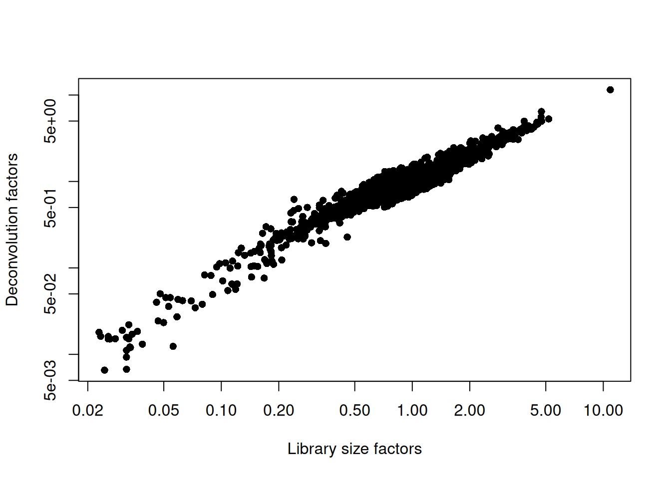
 ``` ``` r plot(librarySizeFactors(sce.pbmc), sizeFactors(sce.pbmc), pch=16, xlab="Library size factors", ylab="Deconvolution factors", log="xy") ```
Relationship between the library size factors and the deconvolution size factors in the PBMC dataset.

(\#fig:unref-unfiltered-pbmc-norm)Relationship between the library size factors and the deconvolution size factors in the PBMC dataset.

## Variance modelling ``` r set.seed(1001) dec.pbmc <- modelGeneVarByPoisson(sce.pbmc) top.pbmc <- getTopHVGs(dec.pbmc, prop=0.1)
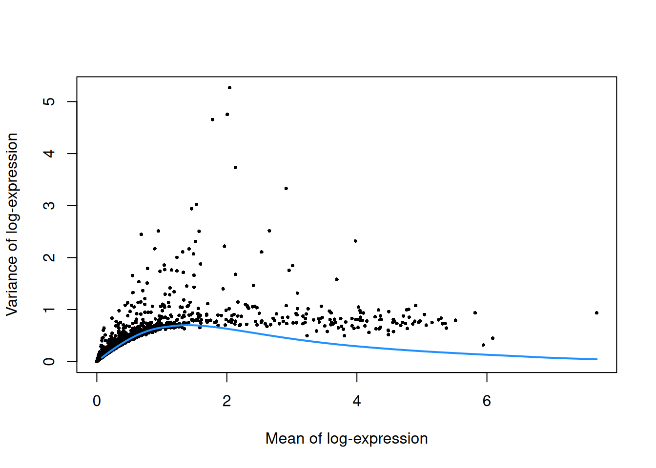
 ``` ``` r plot(dec.pbmc$mean, dec.pbmc$total, pch=16, cex=0.5, xlab="Mean of log-expression", ylab="Variance of log-expression") curfit <- metadata(dec.pbmc) curve(curfit$trend(x), col='dodgerblue', add=TRUE, lwd=2) ```
Per-gene variance as a function of the mean for the log-expression values in the PBMC dataset. Each point represents a gene (black) with the mean-variance trend (blue) fitted to simulated Poisson counts.

(\#fig:unref-unfiltered-pbmc-var)Per-gene variance as a function of the mean for the log-expression values in the PBMC dataset. Each point represents a gene (black) with the mean-variance trend (blue) fitted to simulated Poisson counts.

## Dimensionality reduction ``` r set.seed(10000) sce.pbmc <- denoisePCA(sce.pbmc, subset.row=top.pbmc, technical=dec.pbmc) set.seed(100000) sce.pbmc <- runTSNE(sce.pbmc, dimred="PCA") set.seed(1000000) sce.pbmc <- runUMAP(sce.pbmc, dimred="PCA") ``` We verify that a reasonable number of PCs is retained. ``` r ncol(reducedDim(sce.pbmc, "PCA")) ``` ``` ## [1] 9 ``` ## Clustering ``` r g <- buildSNNGraph(sce.pbmc, k=10, use.dimred = 'PCA') clust <- igraph::cluster_walktrap(g)$membership colLabels(sce.pbmc) <- factor(clust) ``` ``` r table(colLabels(sce.pbmc)) ``` ``` ## ## 1 2 3 4 5 6 7 8 9 10 11 12 13 14 15 16 ## 202 590 523 780 55 359 126 753 46 151 144 77 82 25 17 21 ``` ``` r plotTSNE(sce.pbmc, colour_by="label") ```
Obligatory $t$-SNE plot of the PBMC dataset, where each point represents a cell and is colored according to the assigned cluster.

(\#fig:unref-unfiltered-pbmc-tsne)Obligatory $t$-SNE plot of the PBMC dataset, where each point represents a cell and is colored according to the assigned cluster.

## Interpretation ``` r markers <- findMarkers(sce.pbmc, pval.type="some", direction="up") ``` We examine the markers for cluster 4 in more detail. High expression of _CD14_, _CD68_ and _MNDA_ combined with low expression of _FCGR3A_ (_CD16_) suggests that this cluster contains monocytes, compared to macrophages in cluster 13 (Figure \@ref(fig:unref-mono-pbmc-markers)). ``` r marker.set <- markers[["4"]] as.data.frame(marker.set[1:30,1:3]) ``` ``` ## p.value FDR summary.logFC ## MNDA 0.000e+00 3.953e-323 2.4130 ## RP11-1143G9.4 1.401e-283 2.360e-279 2.6731 ## FCN1 1.047e-269 1.176e-265 2.6884 ## CSTA 8.279e-264 6.974e-260 2.2625 ## VCAN 1.396e-249 9.405e-246 1.8120 ## S100A12 1.765e-212 9.911e-209 2.3921 ## FGL2 1.538e-207 7.401e-204 1.4542 ## LGALS2 2.310e-193 9.729e-190 1.9884 ## MS4A6A 3.077e-192 1.152e-188 1.4849 ## CFD 3.427e-182 1.155e-178 1.4380 ## CD14 2.440e-175 7.475e-172 1.3140 ## CLEC7A 3.806e-174 1.069e-170 1.0823 ## SERPINA1 6.175e-168 1.600e-164 1.4856 ## AIF1 1.025e-167 2.467e-164 2.6619 ## KLF4 5.359e-158 1.204e-154 1.1672 ## TYMP 1.348e-156 2.840e-153 2.0407 ## CFP 5.317e-146 1.054e-142 1.1002 ## NAMPT 4.321e-141 8.089e-138 1.0566 ## IFI30 1.402e-139 2.486e-136 0.9611 ## CD68 3.187e-136 5.369e-133 1.1208 ## MPEG1 4.107e-135 6.589e-132 0.9498 ## CYBB 9.544e-133 1.462e-129 1.1915 ## LGALS3 5.012e-132 7.343e-129 0.9240 ## TNFSF13B 9.896e-130 1.389e-126 1.0572 ## CPVL 2.309e-122 3.112e-119 0.8207 ## CSF3R 2.155e-120 2.793e-117 0.8046 ## CD302 2.855e-118 3.562e-115 0.8382 ## CTSS 1.026e-115 1.235e-112 3.2502 ## BLVRB 1.097e-114 1.275e-111 0.9200 ## GRN 1.043e-113 1.171e-110 1.4442 ``` ``` r plotExpression(sce.pbmc, features=c("CD14", "CD68", "MNDA", "FCGR3A"), x="label", colour_by="label") ```
Distribution of expression values for monocyte and macrophage markers across clusters in the PBMC dataset.

(\#fig:unref-mono-pbmc-markers)Distribution of expression values for monocyte and macrophage markers across clusters in the PBMC dataset.

## Session Info {-}
``` R version 4.5.0 RC (2025-04-04 r88126) Platform: x86_64-pc-linux-gnu Running under: Ubuntu 24.04.2 LTS Matrix products: default BLAS: /home/biocbuild/bbs-3.21-bioc/R/lib/libRblas.so LAPACK: /usr/lib/x86_64-linux-gnu/lapack/liblapack.so.3.12.0 LAPACK version 3.12.0 locale: [1] LC_CTYPE=en_US.UTF-8 LC_NUMERIC=C [3] LC_TIME=en_GB LC_COLLATE=C [5] LC_MONETARY=en_US.UTF-8 LC_MESSAGES=en_US.UTF-8 [7] LC_PAPER=en_US.UTF-8 LC_NAME=C [9] LC_ADDRESS=C LC_TELEPHONE=C [11] LC_MEASUREMENT=en_US.UTF-8 LC_IDENTIFICATION=C time zone: America/New_York tzcode source: system (glibc) attached base packages: [1] stats4 stats graphics grDevices utils datasets methods [8] base other attached packages: [1] scran_1.36.0 EnsDb.Hsapiens.v86_2.99.0 [3] ensembldb_2.32.0 AnnotationFilter_1.32.0 [5] GenomicFeatures_1.60.0 AnnotationDbi_1.70.0 [7] scater_1.36.0 ggplot2_3.5.2 [9] scuttle_1.18.0 DropletUtils_1.28.0 [11] SingleCellExperiment_1.30.0 SummarizedExperiment_1.38.0 [13] Biobase_2.68.0 GenomicRanges_1.60.0 [15] GenomeInfoDb_1.44.0 IRanges_2.42.0 [17] S4Vectors_0.46.0 BiocGenerics_0.54.0 [19] generics_0.1.3 MatrixGenerics_1.20.0 [21] matrixStats_1.5.0 DropletTestFiles_1.17.0 [23] BiocStyle_2.36.0 rebook_1.18.0 loaded via a namespace (and not attached): [1] jsonlite_2.0.0 CodeDepends_0.6.6 [3] magrittr_2.0.3 ggbeeswarm_0.7.2 [5] farver_2.1.2 rmarkdown_2.29 [7] BiocIO_1.18.0 vctrs_0.6.5 [9] memoise_2.0.1 Rsamtools_2.24.0 [11] DelayedMatrixStats_1.30.0 RCurl_1.98-1.17 [13] htmltools_0.5.8.1 S4Arrays_1.8.0 [15] AnnotationHub_3.16.0 curl_6.2.2 [17] BiocNeighbors_2.2.0 Rhdf5lib_1.30.0 [19] SparseArray_1.8.0 rhdf5_2.52.0 [21] sass_0.4.10 bslib_0.9.0 [23] cachem_1.1.0 GenomicAlignments_1.44.0 [25] igraph_2.1.4 mime_0.13 [27] lifecycle_1.0.4 pkgconfig_2.0.3 [29] rsvd_1.0.5 Matrix_1.7-3 [31] R6_2.6.1 fastmap_1.2.0 [33] GenomeInfoDbData_1.2.14 digest_0.6.37 [35] colorspace_2.1-1 dqrng_0.4.1 [37] irlba_2.3.5.1 ExperimentHub_2.16.0 [39] RSQLite_2.3.9 beachmat_2.24.0 [41] labeling_0.4.3 filelock_1.0.3 [43] httr_1.4.7 abind_1.4-8 [45] compiler_4.5.0 bit64_4.6.0-1 [47] withr_3.0.2 BiocParallel_1.42.0 [49] viridis_0.6.5 DBI_1.2.3 [51] HDF5Array_1.36.0 R.utils_2.13.0 [53] rappdirs_0.3.3 DelayedArray_0.34.0 [55] bluster_1.18.0 rjson_0.2.23 [57] tools_4.5.0 vipor_0.4.7 [59] beeswarm_0.4.0 R.oo_1.27.0 [61] glue_1.8.0 h5mread_1.0.0 [63] restfulr_0.0.15 rhdf5filters_1.20.0 [65] grid_4.5.0 Rtsne_0.17 [67] cluster_2.1.8.1 gtable_0.3.6 [69] R.methodsS3_1.8.2 metapod_1.16.0 [71] BiocSingular_1.24.0 ScaledMatrix_1.16.0 [73] XVector_0.48.0 ggrepel_0.9.6 [75] BiocVersion_3.21.1 pillar_1.10.2 [77] limma_3.64.0 dplyr_1.1.4 [79] BiocFileCache_2.16.0 lattice_0.22-7 [81] FNN_1.1.4.1 rtracklayer_1.68.0 [83] bit_4.6.0 tidyselect_1.2.1 [85] locfit_1.5-9.12 Biostrings_2.76.0 [87] knitr_1.50 gridExtra_2.3 [89] bookdown_0.43 ProtGenerics_1.40.0 [91] edgeR_4.6.0 xfun_0.52 [93] statmod_1.5.0 UCSC.utils_1.4.0 [95] lazyeval_0.2.2 yaml_2.3.10 [97] evaluate_1.0.3 codetools_0.2-20 [99] tibble_3.2.1 BiocManager_1.30.25 [101] graph_1.86.0 cli_3.6.4 [103] uwot_0.2.3 munsell_0.5.1 [105] jquerylib_0.1.4 Rcpp_1.0.14 [107] dir.expiry_1.16.0 dbplyr_2.5.0 [109] png_0.1-8 XML_3.99-0.18 [111] parallel_4.5.0 blob_1.2.4 [113] sparseMatrixStats_1.20.0 bitops_1.0-9 [115] viridisLite_0.4.2 scales_1.3.0 [117] purrr_1.0.4 crayon_1.5.3 [119] rlang_1.1.6 cowplot_1.1.3 [121] KEGGREST_1.48.0 ```